During your exam, if you see questions about the Box-Cox transformation, remember that it is a method that can perform many power transformations (according to a lambda parameter), and its end goal is to make the original distribution closer to a normal distribution.
Just to conclude this discussion regarding why mathematical transformations can really make a difference to ML models, here is an example of exponential transformations.
Suppose you have a set of data points, such as those on the left-hand side of Figure 4.7. Your goal is to draw a line that will perfectly split blue and red points. Just by looking at the original data (again, on the left-hand side), you know that your best guess for performing this linear task would be the one you can see in the same figure. However, the science (not magic) happens on the right-hand side of the figure! By squaring those numbers and plotting them in another hyper plan, you can perfectly separate each group of points.
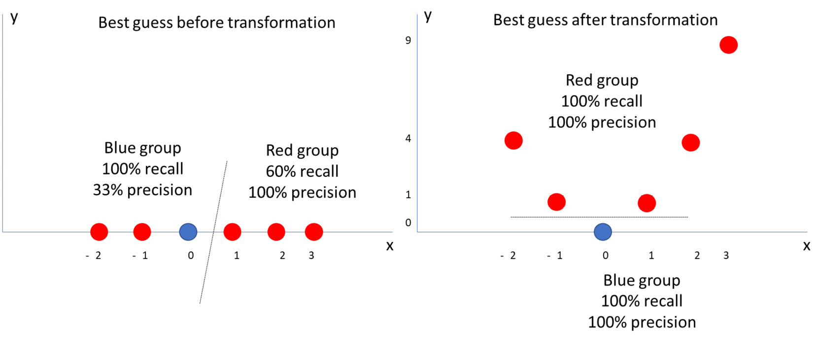
Figure 4.7 – Exponential transformation in action
You might be thinking that there are infinite ways in which you can deal with your data. Although this is true, you should always take the business scenario you are working on into account and plan the work accordingly. Remember that model improvements or exploration is always possible, but you have to define your goals (remember the CRISP-DM methodology) and move on.
By the way, data transformation is important, but it is just one piece of your work as a data scientist. Your modeling journey still needs to move to other important topics, such as missing values and outliers handling. However, before that, you may have noticed that you were introduced to Gaussian distributions during this section, so why not go deeper into it?
Although the Gaussian distribution is probably the most common distribution for statistical and machine learning models, you should be aware that it is not the only one. There are other types of data distributions, such as the Bernoulli, binomial, and Poisson distributions.
The Bernoulli distribution is a very simple one, as there are only two types of possible events: success or failure. The success event has a probability p of happening, while the failure one has a probability of 1-p.
Some examples that follow a Bernoulli distribution are rolling a six-sided die or flipping a coin. In both cases, you must define the event of success and the event of failure. For example, assume the following success and failure events when rolling a die:
You can then say that there is a p probability of success (1/6 = 0.16 = 16%) and a 1-p probability of failure (1 – 0.16 = 0.84 = 84%).
The binomial distribution generalizes the Bernoulli distribution. The Bernoulli distribution has only one repetition of an event, while the binomial distribution allows the event to be repeated many times, and you must count the number of successes. Continue with the prior example, that is, counting the number of times you got a 6 out of our 10 dice rolls. Due to the nature of this example, binomial distribution has two parameters, n and p, where n is the number of repetitions and p is the probability of success in every repetition.
Finally, a Poisson distribution allows you to find a number of events in a period of time, given the number of times an event occurs in an interval. It has three parameters: lambda, e, and k, where lambda is the average number of events per interval, e is the Euler number, and k is the number of times an event occurs in an interval.
With all those distributions, including the Gaussian one, it is possible to compute the expected mean value and variance based on their parameters. This information is usually used in hypothesis tests to check whether some sample data follows a given distribution, by comparing the mean and variance of the sample against the expected mean and variance of the distribution.
You are now more familiar with data distributions, not only Gaussian distributions. You will keep learning about data distributions throughout this book. For now, it is time to move on to missing values and outlier detection.
Acedexam Training Policies
Learning resources
Other resources
Our Training Providers